Backtesting Random Trading Signals: From Chaos to Code

I tested a strategy using a random generator. And let's see how it performs based on such randomly generated signals.

Not true-random

We will be using a random seed source number of 42. This is to achieve consistent results on re-runs of the backtest. If we seed it with a timestamp, the results will be different at each run.

var rng = rand.New(rand.NewSource(42))

Calculations of the stop loss and take profit targets

For simplicity, I use points based on NQ=20000. This creates a percentage-based stop loss across multiple years.

For example, when I say SL=50, the stop loss will be set at 50 points based on 20000. That is 0.25%. To avoid any confusion, this means that if the entry price at NQ is 20000, then the stop price would be at 19950. If NQ is 21000, then the stop price would be 20947 (21000 - 53), where 53 represents the ceiling value based on a 0.25% margin.

Similarly, the take profit points are also recalculated based on the entry price.

Unless explicitly mentioned, the stop loss will be set at 50 points (of 20k)

Strategy

We will be backtesting the trades with the NQ Futures E-mini contract, and we will take the entry right at the open, i.e., 9:30 AM Eastern Time.

The backtesting is performed from 2008 to early 2025, using a 1-minute dataset.

1. Entry time is at standard market open only.
2. Exit time, if none of the SL/TP are hit, is market close hours. Usually 16.00 hours. On holidays, the futures market may have short trading hours, and we use that market's close.
3. Intraday only. No overnight holding.
4. SL and TP as defined

The profits are calculated based on the actual exit price; we do not arbitrarily assume whether a take-profit is hit or not. For larger take-profits, it is very likely to close at a smaller profit or a loss.

Random signal

And the random signal works like this:

1. Generate a random number between and inclusive of the range (0 to 999)
2. If the number is divisible by 2, then we have a long signal
3. Otherwise, we have a short signal

func getRandomSignal() int {
	rndno := rng.Intn(1000)

	if rndno%2 == 0 {
		return 1
	}
	return -1
}

Yes, it is that simple.

Backtest results

Next, we test with different stop losses and the take profit levels

SL=50. TP=50.

(Read above how points are adjusted based on the underlying)

This is a slightly negative reward-to-risk ratio. Why negative? Slippage and commissions

In practice, even if you use "Bid/Ask" limit orders, you will also see some entry slippage because the price moves very fast at the opening bell.

Win rate: 51.02%

The results are not so exciting. It took off somewhere after 2020.

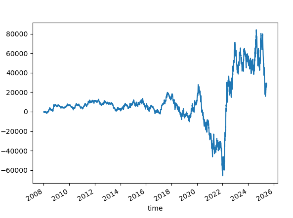
SL=50. TP=150.

Win rate: 31.27%

The results are slightly better. It often remained positive. There was a drawdown between 2019 and 2020, and then it took off. However, it has not been good; it has stayed flat for many years.

Despite the lower win rate, the benefit of a high 3:1 reward-risk ratio is evident.

However, the lower win rate might be unsettling. So, let us see if we can lower the profit targets and achieve a better win rate.

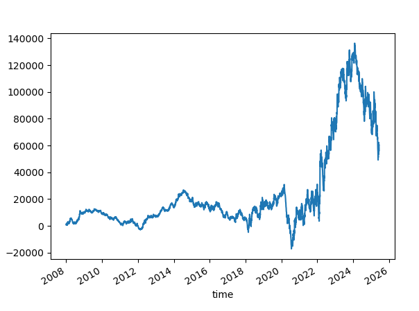
SL=50. TP=110.

Win rate: 35.6%

Similar, but with lower profit and a better win rate.

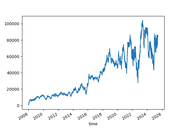
SL=50. TP = Not Set or 1000

We let the winners run. The TP is unreasonably high and never occurs.

Win rate is 27%.

Win rate is pretty low, yet the reward-risk magic works here. And we have an upward-sloping profit curve.

NOTE: TP=1000 is 5%. Means it is unlikely to hit the take-profit. All profit calculations are based on the intraday exit price when the market closes.

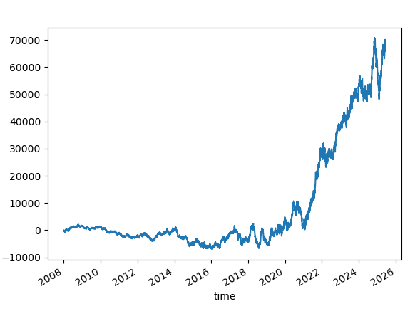
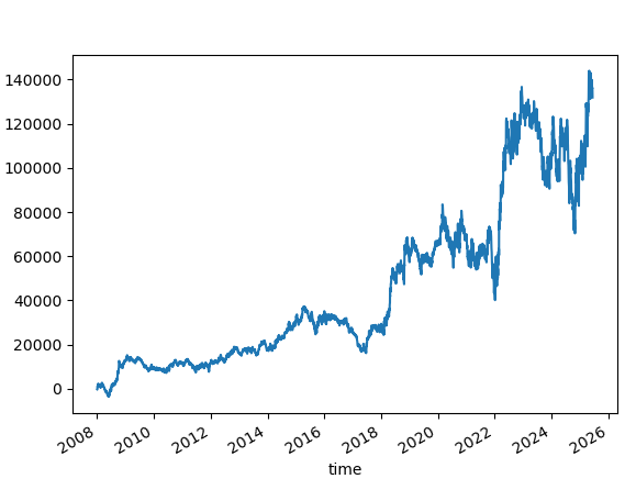
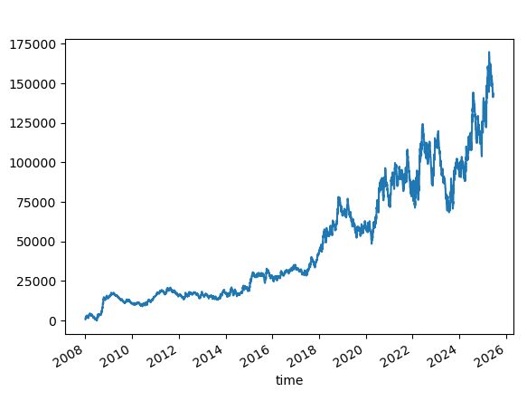
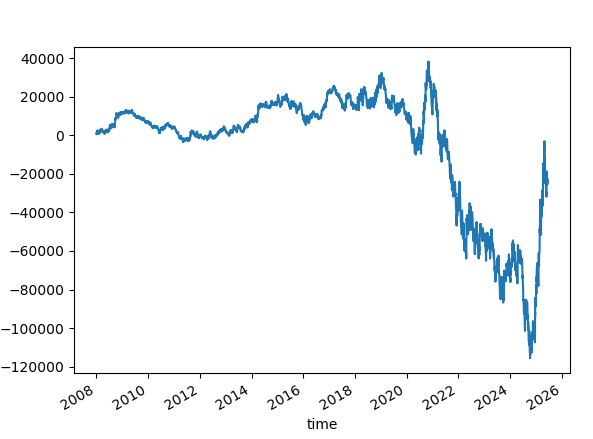
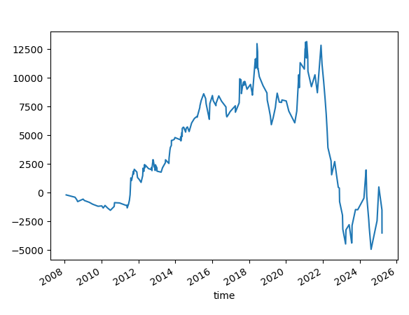
SL=100. TP = Not Set

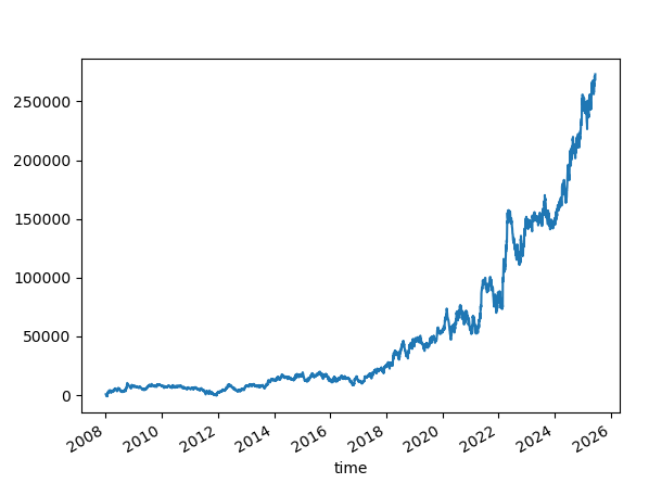
Win rate is 38.71%

This one is interesting. After 2012, we have an upward slope on the profit curve.

The value of NQ is smaller in the earlier years, and therefore, the profit curve appears relatively flat in the results above.

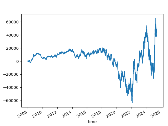
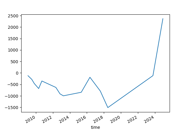
Changing the random seed

But what happens if the random seed is changed to something else, let's say 41?

With SL=100, TP=Not Set, where we initially saw good results with 42, the current results with 41 are significantly worse.

No superstition, please.

Why did I use 42 as a seed source? It is common in machine learning, and I just carried over the seed here. Here's the fascinating story behind it.

The story behind ‘random.seed(42)’ in machine learning

Answer to the great question of “Life, the universe, and everything”!

Geek CultureNazia Nafis

Let's see another experiment with the random seed 42. Let's skip the first few numbers. The results vary; they are not as bad as changing the seed, but not something you would like to see on a profit curve.

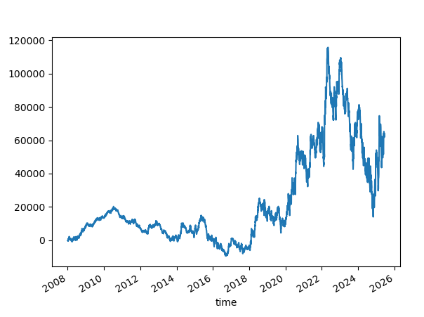
Trusting that a particular random seed works, when started at a specific date, is superstitious. And yet, it may continue to work in the future.

Ensemble of Randoms

So what happens if we have an ensemble of random number generators?

The idea is this:

1. Create 100 random number generators, seeded from 1 to 100.
2. Generate the random number and the signal using the same logic as above, but now do it for each of the generators.
3. Take a majority vote, and use that as a signal. Therefore, if we have 60 short signals and 40 long signals, we will use Short as a signal

var rngs []*rand.Rand

func init() {
  // Initialize multiple random number generators with different seeds
  for i := 0; i < 100; i++ {
    rngs = append(rngs, rand.New(rand.NewSource(int64(i+1))))
  }
}

func getRandomSignal() int {

	// Get from an ensemble of random number generators
	longCounts := 0.0
	shortCounts := 0.0
	for _, r := range rngs {
		rndno := r.Intn(1000)
		if rndno%2 == 0 {
			longCounts++
		} else {
			shortCounts++
		}
	}
	//....
	signal := 0
	if longCounts > shortCounts {
		signal = 1 // Buy signal
	} else if shortCounts > longCounts {
		signal = -1 // Sell signal
	} else {
		signal = 0 // No signal
	}

	return signal

}

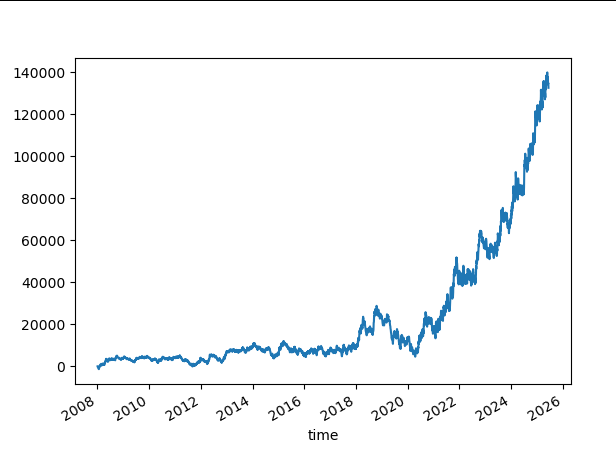
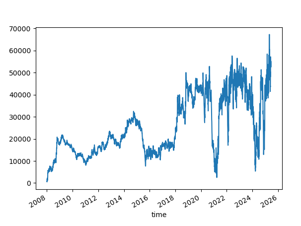
SL=100.TP=Not Set

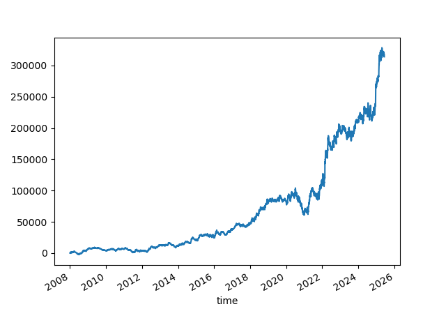
An attempt at reducing the stop loss.

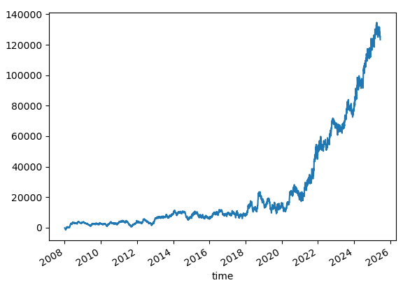
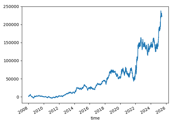
SL=50.TP=Not Set

But is this just the reward-risk magic?

Let's try reversing the signal with SL=100, TP=None.

Well, it could be, but it doesn't seem to be just that.

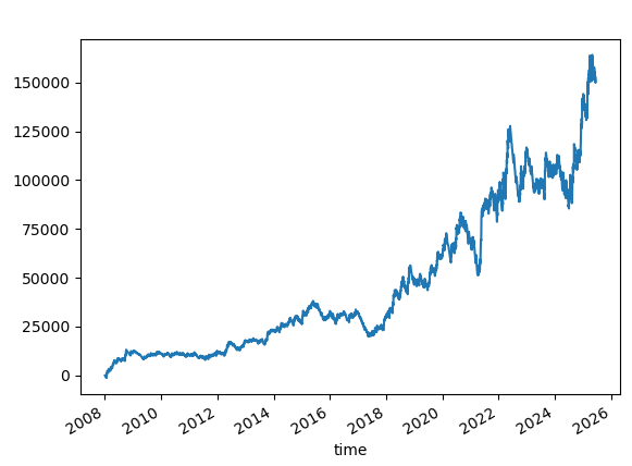
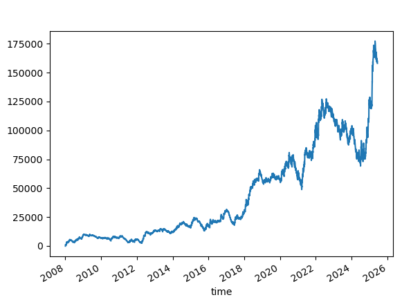
Skipping a few signals

What if we skip a few signals? Like we did before.

We continue with SL=100 and TP=None.

Increasing Ensemble size to 10,000

Let's try using an ensemble of 10000

Increasing the size doesn't help as much. Let us look at the probabilities.

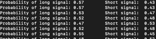
The probability of Short is just the opposite of the Long.

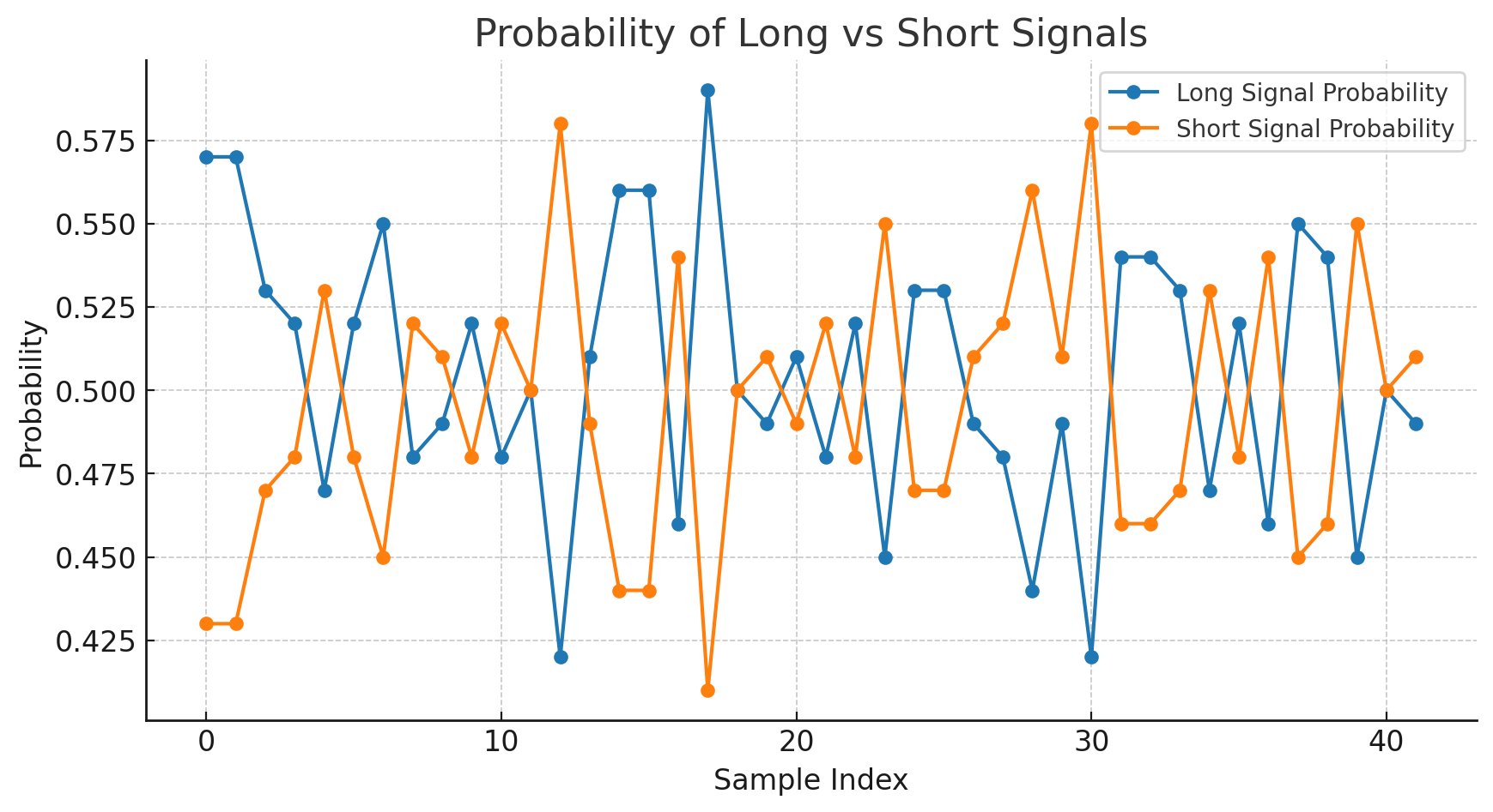
But when we see an ensemble size of 10000, the variation is tiny and hovers just about 50%.

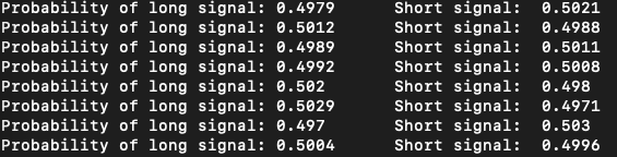
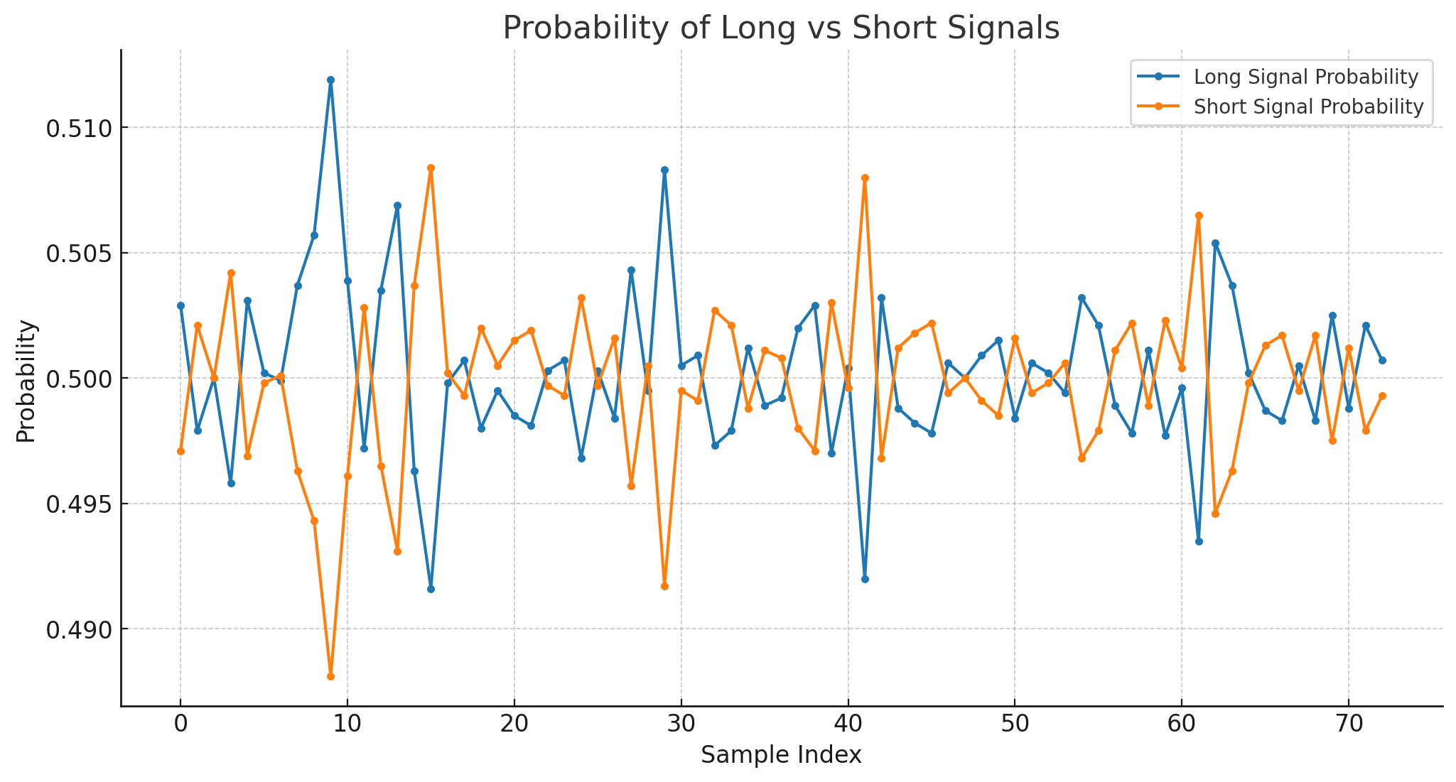
With a larger ensemble size, we see spikes on the probabilities, but the range on those is very small. Therefore, there is a lot of noise in the higher ensemble sizes.

Can we filter out the noise and backtest the results?

For size = 10000, one standard deviation is 0.005.

• 68% of the time → long probability will be between 0.495 and 0.505.
• 95% of the time → long probability will be between 0.49 and 0.51.
• 99.7% of the time → long probability will be between 0.485 to 0.515.

What if we only used signals when long probability is breaching or touching the extremes of 0.485 to 0.515.

if probability >= 0.515 || probability <= 0.485 {
	return signal
} else {
	signal = 0 // No signal no trade
}

I want to point out that most of the cases that are displayed above have higher reward-to-risk ratios. We control the risk. We are not dealing with a negative reward risk. We are taking trades right at the open and holding them for a very long time.

Illusion of Edge/Skill

It looks like there is an edge in the filtering, but it's not. The underlying signal is random, and therefore, the win expectancy is going to be 50%. The “range filter” is a trade frequency filter, not a predictive edge. Without a real signal inside the generators, there’s nothing to exploit — it’s just data-snooping if you see an edge in backtest.

The in-sample profit slope may not align with out-of-sample tests. In the entire exercise above, I did not split the data into train-validation-test datasets, and it is easy to see why we could be experiencing overfitting.

But what if the underlying signal isn’t purely random? And what exactly do we mean by “pure randomness”? Something worth pondering.

Disclaimer
The information, strategies, and examples provided in this article are intended solely for educational and entertainment purposes. They do not constitute financial, investment, or trading advice. Past performance—whether simulated or actual—does not guarantee future results. Trading involves significant risk of loss and is not suitable for every investor. Always conduct your own research and consult with a licensed financial advisor before making any trading or investment decisions.

Assumptions: The dataset is unadjusted continuous futures 1-minute data for NQ. Slippages and commissions are accounted for in the backtest. Commissions are assumed to be average, which a retail trader can reasonably expect to get. With NQ, 1 point is assumed to be 4 ticks. 1 tick is 0.25, and 1 point is equal to $20 change in P&L. This assumption may not hold for past trades - we have assumed simplicity here. Right-at-open orders may not exactly fill. In practice, placing a best bid/ask order 5-7 seconds earlier is preferable, as it can result in either positive or negative minor slippage, but ultimately nets to zero over many trades. For intrabar ambiguity, we always assume that SL hits first. We are using percentage-based SL and TP for simplicity - volatility-based levels are not used here, but note that 17 years of data will see a lot of variance in volatility. The backtest code is written in Go, and we use Python for analyzing results.

Want to see more of such experiments with randomness? Leave a comment below!